🏁 Automatically Detect Encroachment in Penalty Kicks!

Penalty Kicks are one of football's most exciting and important moments, which is why it is so important that the referee gets the call right. This project aims to leverage Computer Vision and Machine Learning to automatically detect encroachment during penalty kicks. pen1 Our starting point

What is encroachment?

Encroachment is when players (attackers or defenders) enter the box before the ball is kicked by the penalty taker.

Why is this a problem?

This is a problem because if undetected, players who enter the box prematurely will gain an unfair advantage reaching the loose ball.

Why is this project needed?

The inspiration for this project came when undetected encroachment cost Borussia Dortmund the game against Chelsea in the 2022-2023 Champions League. Referees often overlook encroachment while watching the goalkeepers and seeing if they stay on their line. Such an autonomous tool could create a more authentic refereeing experience, also eliminating human error.

🔑 Key Features

Player and Ball Tracking

The project employs object detection and tracking algorithms to identify and track the positions of players on the field throughout the Penalty sequence. pen2

💻 Code

For the intial player detection, we utilized a pre trained YOLOv8 model

from ultralytics import YOLO
# import model from pretrained weights file
model = YOLO("yolov8m.pt")
 
# read a frame from video
ret, frame = cap.read()
 
# run model on the frame
results = model(frame, device="mps")

Then we need to extract the information we want from the model's results, which will be the bounding boxes and the classes

bounding_boxes = np.array(result.boxes.xyxy.cpu(), dtype="int")
classes = np.array(result.boxes.cls.cpu(), dtype="int")

Now, we need to label the frame with the information we gathered

for cls, bbox in zip(classes, bounding_boxes):
        # label players
        if cls == 0:
            (x, y, x2, y2) = bbox
            cv2.rectangle(frame, (x, y), (x2, y2), (0, 0, 225), 2)
            cv2.putText(frame, "Player", (x, y - 5), cv2.FONT_HERSHEY_PLAIN, 2, (0, 0, 225), 2)
        # label ball
        if cls == 32:
            (x, y, x2, y2) = bbox
            cv2.rectangle(frame, (x, y), (x2, y2), (0, 0, 225), 2)
            cv2.putText(frame, "Ball", (x, y - 5), cv2.FONT_HERSHEY_PLAIN, 2, (0, 0, 225), 2)

Segmentation and Team Classification

The program also detects players more finely and additionally, and classifies them based on which team they belong to. pen3 Notice the finer bounding boxes as well as the blue rectangle within. The player's jerseys RGB value is displayed above them, and colored in that same value

💻 Code

First, let's look at segmentation. YOLO originally creates bounding boxes for each objet, but as seen above, these boxes come as a rectangle. Sometimes, we'll need more detail, which is when we want to use YOLO segmentation. I'll let the picture below show you the difference.

Segmentation example

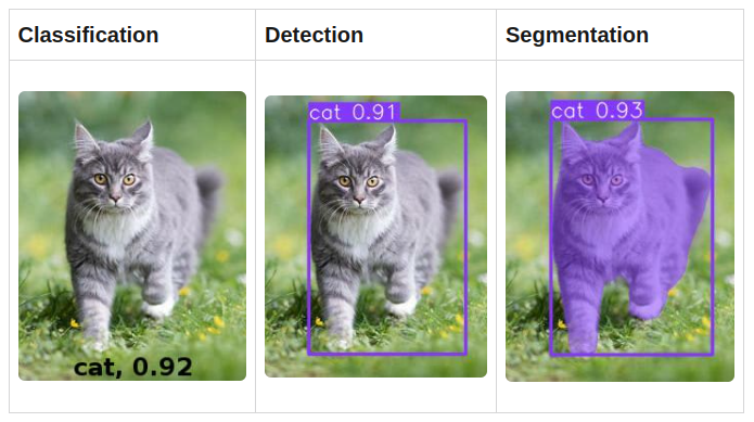
Image from freecodecamp.org

We can now use YOLO Segmentation to acquire finer bounding boxes for the players and then, using the more precise segmentation, an algorithm to identify which team each player belongs to.

Let's implement segmentation:

# import yolo segmentation model and use pre trained weights file
from yolo_segmentation import YOLOSegmentation
yolo_seg = YOLOSegmentation("yolov8m-seg.pt")
 
# bounding_boxes - the bounding boxes
# classes - the object classes
# segementation - the values to segment within the boxes
# scores - the confidence score of the detection
bounding_boxes, classes, segmentations, scores = yolo_seg.detect(frame)

Now let's create a function to pull the most dominant color from within a box

def get_average_color(a):
    return tuple(np.array(a).mean(axis=0).mean(axis=0).round().astype(int))

Finally, lets put our loop together to annotate the segmentations and common color! Notice that within the loop, we'll redact a portion of the original segmentation to have the new frame be as much jersey as possible. This redacted portion is the original frame. Then we'll find the average color.

for bbox, class_id, seg, score in zip(bounding_boxes, classes, segmentations, scores):
        if class_id == 0:
            (x, y, x2, y2) = bbox
 
            # redact a frame that encompasses most of the player's jersey
            minY = np.max(seg[:, 1])
            bottomVal = int(2*(minY - seg[0][1])/3 + seg[0][1])
            
            a = frame2[seg[0][1]:bottomVal, seg[0][0]:seg[len(seg)-1][0]]
 
            cv2.polylines(frame, [seg], True, (0, 0, 225), 2)
            cv2.rectangle(frame, (seg[0][0], seg[0][1]), (seg[len(seg)-1][0], bottomVal), (225, 0, 0), 2)
            cv2.putText(frame, str(get_average_color(a)), (x, y-5), cv2.FONT_HERSHEY_PLAIN, 2, (int(get_average_color(a)[0]), int(get_average_color(a)[1]), int(get_average_color(a)[2])), 4)

Penalty Box Detection

The program also employs detection of the penalty box through various techniques. In this case we'll be using OpneCV contours and Hough Line Transformations.

pen4 Notice how every straight line is highlighted

💻 Code

So we saw how every line in the image was highlighted blue. That's the magic of contours. Let's get into how it works:

Let's look at the code for contours.

thresh = cv2.adaptiveThreshold(Y,255,cv2.ADAPTIVE_THRESH_MEAN_C, cv2.THRESH_BINARY_INV,35,5)
 
contours, hierarchy = cv2.findContours(thresh, cv2.RETR_EXTERNAL, cv2.CHAIN_APPROX_NONE)

First, we'll apply a threshold. The threshold signifies what distance a line must be to be counted as a contour line. A larger value will only highlight longer lines while a smaller value will highlight more. Then using the threshold, we then use OpenCV's findcontours function to grab a list of our contours - all the ones in the frame. Next, as usual, we'll draw them on the frame.

x=[]
    for i in range(0, len(contours)):
        if cv2.contourArea(contours[i]) > 2400:
            x.append(contours[i])
 
 cv2.drawContours(frame, x, -1, (255,0,0), 2)

You'll see we add an additional check for the length of the contour in pixels, before appending it to list x that we eventually draw.

To take it a step further, let's look at Hough Line Transformations. These help identify lines even through breakage or inorganic shapes.

To perform Hough Line Transformations, first we need to preprocess the frame:

# grayscale the frame
gs = cv2.cvtColor(frame, cv2.COLOR_BGR2GRAY)
 
# utilize canny to get edges in frame
edges = cv2.Canny(gs, 50, 150, apertureSize=3)
 
# perform hough line tranformation to selectively get edges based on certain parameters.
lines = cv2.HoughLinesP(edges, 1, np.pi / 180, threshold=100, minLineLength=100, maxLineGap=10)

The process requires the image to be grayscale, so that is what we do first. Then we apply the canny edge detecting algorithm on the grayscale frame to grab the edges. Next, we apply Hough Line Transformation on our edges to selectively choose which ones we want.

Now, let's have some fun filtering.

penalty_box_lines = []
    semicircle_points = []
 
    for line in lines:
        if len(line) == 4:
            x1, y1, x2, y2 = line[0]
        else:
            x1, y1, dx, dy = line[0]
            x2, y2 = x1 + dx, y1 + dy
 
        angle = np.arctan2(y2 - y1, x2 - x1) * 180.0 / np.pi
 
        if 80 <= angle <= 100 and y1 > frame.shape[0] / 2:
            penalty_box_lines.append(line)
        elif angle == 0 and x1 > frame.shape[1] / 2:
            semicircle_points.append((x1, y1))
            semicircle_points.append((x2, y2))
 
    for line in penalty_box_lines:
        x1, y1, x2, y2 = line[0]
        cv2.line(frame, (x1, y1), (x2, y2), (0, 255, 0), 2)
 
    if len(semicircle_points) == 2:
        center_x = int((semicircle_points[0][0] + semicircle_points[1][0]) / 2)
        center_y = int((semicircle_points[0][1] + semicircle_points[1][1]) / 2)
        radius = int(np.sqrt((semicircle_points[0][0] - semicircle_points[1][0]) ** 2 +
                             (semicircle_points[0][1] - semicircle_points[1][1]) ** 2) / 2)
 
        cv2.circle(frame, (center_x, center_y), radius, (0, 255, 0), 2)

This is a lot to explain but just sift through this code a little bit and you can break it down! This portion was just playing around with the angles until we found something that worked best.

🪴 Areas of Improvement

Real-Time Video Analysis: Achieving real time video analysis at a good frame rate is a big goal. The program is very computationally expensive, so with the right hardware, I'm sure it can be done, but that is something to test and eventually implement in the future.
Deep Sort: Deepsort assigns unqique IDs to each player and tracks them throughout the video. This would be a great addition to the system as we could then tell which player is commiting the infraction.

🚀 Further Uses

Goalkeeper checking: Eventually, the project can also be extended to track goalkeepers and making sure that they stay on their line.
Player Jersey Number Recognition: The system could later utilizes Optical Character Recognition (OCR) techniques to read the jersey numbers of players on the field. This allows an alternate way to identify the offending player. This one is highly variable on camera angle however.

💻 Technology

Ultralytics
OpenCV
NumPy
YoloV8 / YoloSegmentation