🏁 Automate tennis match analysis using the power of computer vision.
CourtCheck leverages advanced computer vision techniques to accurately track tennis ball movements and court boundaries in tennis matches. This project aims to provide real-time insights and automated decision-making in tennis, reducing human error and enhancing the accuracy of in/out calls. CourtCheck integrates Python, machine learning, and computer vision to create a seamless and efficient system for tennis match analysis.

🔑 Process & Key Features
1. 🔎 Court Detection
CourtCheck employs keypoint detection algorithms to identify and track the tennis court's boundaries, ensuring accurate mapping and analysis of the court's dimensions.
a. 📑 Annotation
We began by annotating images using OpenCV in the COCO format, generating JSON files for each annotated image. The OpenCV Annotation Tool provides an excellent interface for image annotation and export in various formats. It also features an interpolation tool that allows the use of a skeleton to label key frames, which can be interpolated over consecutive frames in the video.
You can find the annotations here.
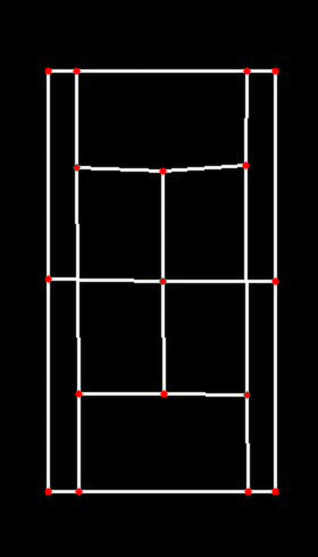
Each label in the skeleton represents a keypoint on the tennis court, identifying an important corner or intersection of lines that are crucial for the overall court detection when training the model. Here are the keypoints and their corresponding labels:
| Keypoint | Label | Keypoint | Label | Keypoint | Label |
|---|---|---|---|---|---|
| BTL | Bottom Top Left | ITM | Inner Top Middle | ITR | Inner Top Right |
| BTLI | Bottom Top Left Inner | IBR | Inner Bottom Right | NL | Net Left |
| BTRI | Bottom Top Right Inner | NR | Net Right | BBL | Bottom Bottom Left |
| BTR | Bottom Top Right | NM | Net Middle | IBL | Inner Bottom Left |
| BBR | Bottom Bottom Right | ITL | Inner Top Left | IBM | Inner Bottom Middle |
| BBRI | Bottom Bottom Right Inner | BBLI | Bottom Bottom Left Inner |
b. 🤖 Training the Model
We utilized the A100 Nvidia GPU on Google Colab to train our Detectron2 model on different types of datasets. These datasets included varying court surfaces and slightly different camera angles to ensure robustness and generalizability of the model. Below, we explain the process and provide the code used for training the model incrementally with mixed datasets.
Below is an overview of the Detectron2 architecture:
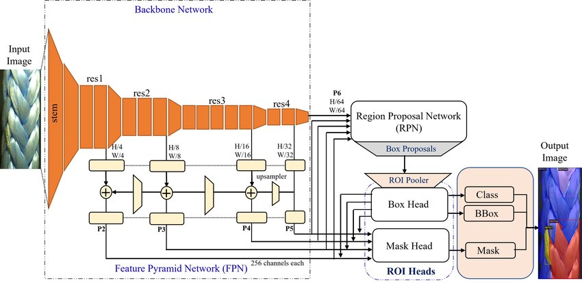
We used the COCO-Keypoints/keypoint_rcnn_R_50_FPN_3x.yaml configuration file because it is specifically designed for keypoint detection tasks. The keypoint_rcnn_R_50_FPN_3x.yaml configuration is well-suited for this task because it includes a pre-trained ResNet-50 backbone that provides strong feature extraction capabilities, coupled with a Feature Pyramid Network (FPN) that helps detect objects at multiple scales. This combination ensures that the model can accurately identify and track the key points on the tennis court, providing precise court boundary detection and enabling accurate in/out call determinations.
c. 🧬 Model Code
The code below sets up and trains the Detectron2 model using multiple datasets:
- Dataset Registration: Registers the training and validation datasets.
- COCO Instance Registration: Registers the datasets in COCO format.
- Metadata Configuration: Configures metadata for keypoints, keypoint flip map, and skeleton.
- Configuration Setup: Sets up the model configuration, including dataset paths, data loader workers, batch size, learning rate, maximum iterations, learning rate decay steps, and checkpoint period.
- Trainer Initialization and Training: Initializes a custom trainer and starts or resumes the training process.
You can find model training in the Google Colab Notebook here.
# Function to set up and train the model with mixed datasets incrementally
def train_model(max_iter, resume=False):
    register_datasets(train_json_files, train_image_dirs, "tennis_game_train")
    register_datasets(val_json_files, val_image_dirs, "tennis_game_val")

    register_coco_instances(f"tennis_game_train", {}, train_json_files, train_image_dirs)
    register_coco_instances(f"tennis_game_val", {}, val_json_files, val_image_dirs)

    MetadataCatalog.get(f"tennis_game_train").keypoint_names = keypoint_names
    MetadataCatalog.get(f"tennis_game_train").keypoint_flip_map = keypoint_flip_map
    MetadataCatalog.get(f"tennis_game_train").keypoint_connection_rules = skeleton

    MetadataCatalog.get(f"tennis_game_val").keypoint_names = keypoint_names
    MetadataCatalog.get(f"tennis_game_val").keypoint_flip_map = keypoint_flip_map
    MetadataCatalog.get(f"tennis_game_val").keypoint_connection_rules = skeleton

    cfg = get_cfg()
    cfg.merge_from_file("/content/drive/MyDrive/ASA Tennis Bounds Project/models/court_detection_model/detectron2/configs/COCO-Keypoints/keypoint_rcnn_R_50_FPN_3x.yaml")
    cfg.DATASETS.TRAIN = tuple([os.path.basename(f).split('.')[0] for f in train_json_files])
    cfg.DATASETS.TEST = tuple([os.path.basename(f).split('.')[0] for f in val_json_files])
    cfg.DATALOADER.NUM_WORKERS = 4
    cfg.SOLVER.IMS_PER_BATCH = 4  # Increase if you have more GPU memory
    cfg.SOLVER.BASE_LR = 0.0001  # Lower learning rate for more careful training
    cfg.SOLVER.MAX_ITER = max_iter  # Total number of iterations
    cfg.SOLVER.STEPS = [int(max_iter*0.75), int(max_iter*0.875)]  # Decay learning rate
    cfg.SOLVER.GAMMA = 0.1  # Decay factor
    cfg.SOLVER.CHECKPOINT_PERIOD = 20000  # Save a checkpoint every 20000 iterations
    cfg.MODEL.ROI_HEADS.BATCH_SIZE_PER_IMAGE = 256  # Increase for more stable gradients
    cfg.MODEL.ROI_HEADS.NUM_CLASSES = 11  # Your dataset has 11 classes

    output_dir = f"/content/drive/MyDrive/ASA Tennis Bounds Project/models/court_detection_model/detectron2/game_model"
    cfg.OUTPUT_DIR = output_dir
    os.makedirs(cfg.OUTPUT_DIR, exist_ok=True)

    trainer = TrainerWithEval(cfg)
    trainer.resume_or_load(resume=resume)
    trainer.train()

# Training parameters
custom_iter = 50000  # Adjust this to your custom number of iterations per session
max_iter = last_iter + custom_iter  # Change this for the number of iterations per session

# Execute to train model
train_model(max_iter, resume=True)
2. 📽️ Post Processing
After training the model, the next crucial step is post-processing the results to ensure accurate and meaningful outputs. Post-processing involves refining the model's predictions and visualizing the detected key points on the tennis court for better interpretation and analysis. The described code snippets below are from court_detection.py.
a. 🖼️ Visualizing the Court on the Main Frame
To accurately visualize the tennis court on the main video frame, we start by detecting key points on the court using the trained model. These key points correspond to specific locations on the court, such as the corners and intersections of lines. Visualizing these key points on the frame helps us understand how well the model is detecting the court's structure.
i. Extracting Key Points from the Model
The court detection model (court_predictor) outputs instances that include predicted key points. These key points are stored in an array where each element corresponds to a specific point on the court, identified by its (x, y) coordinates.
Here's how the key points are extracted:
outputs = court_predictor(img)
instances = outputs["instances"]

if len(instances) > 0:
keypoints = instances.pred_keypoints.cpu().numpy()[0]
else:
keypoints = np.zeros((17, 3))
outputs["instances"]: This contains all detected instances in the frame, including the detected court.instances.pred_keypoints.cpu().numpy()[0]: This extracts the key points of the detected court. The key points are converted from a tensor to a numpy array for further processing.
If no key points are detected, a default array of zeros is used to avoid errors in subsequent processing.
ii. Visualizing Key Points and Court Lines
Once the key points are extracted, the next step is to visualize them by drawing polylines between the points that align with the court lines and boundaries. These lines help in creating a clear and precise representation of the tennis court structure. Here are the specific polylines to be drawn:
lines = [
    ("BTL", "BTLI"), ("BTLI", "BTRI"), ("BTL", "NL"), ("BTLI", "ITL"),
    ("BTRI", "BTR"), ("BTR", "NR"), ("BTRI", "ITR"), ("ITL", "ITM"), ("ITM", "ITR"),
    ("ITL", "IBL"), ("ITM", "NM"), ("ITR", "IBR"), ("NL", "NM"), ("NL", "BBL"),
    ("NM", "IBM"), ("NR", "BBR"), ("NM", "NR"), ("IBL", "IBM"),
    ("IBM", "IBR"), ("IBL", "BBLI"), ("IBR", "BBRI"), ("BBR", "BBRI"),
    ("BBRI", "BBLI"), ("BBL", "BBLI"),
]
Each pair in the lines list represents two key points between which a line will be drawn. These lines outline the court's structure on the video frame.
The visualize_predictions function is essential for visualizing model predictions on an input image. Here are two key parts of the function:
outputs = predictor(img)
v = Visualizer(
    img[:, :, ::-1],
    metadata=MetadataCatalog.get("tennis_game_train"),
    scale=0.8,
    instance_mode=ColorMode.IMAGE,
)
instances = outputs["instances"].to("cpu")

if len(instances) > 0:
    max_conf_idx = instances.scores.argmax()
    instances = instances[max_conf_idx : max_conf_idx + 1]

out = v.draw_instance_predictions(instances)
keypoints = instances.pred_keypoints.numpy()[0]Visualizer: This tool is used to overlay the detected key points and lines on the original image.draw_instance_predictions: This function draws the visual elements on the frame, including key points and the connecting lines.
This process results in a visual overlay of the court on the original video frame, allowing for immediate visual verification of the court detection accuracy.
To ensure that the detected key points on the tennis court are stable and less jittery, especially when dealing with video frames, we use a stabilization technique. This involves averaging the positions of detected key points over a history of frames.
Key Point History Initialization
keypoint_history = {name: deque(maxlen=10) for name in keypoint_names}We initialize a dictionary called keypoint_history where each key is a key point name, and the value is a deque (double-ended queue) with a maximum length of 10. This deque will store the positions of each key point over the last 10 frames.
Stabalizing Keypoints
def stabilize_points(keypoints):
    stabilized_points = []
    for i, keypoint in enumerate(keypoints):
        keypoint_history[keypoint_names[i]].append(keypoint[:2])
        if len(keypoint_history[keypoint_names[i]]) > 1:
            stabilized_points.append(
                np.mean(np.array(keypoint_history[keypoint_names[i]]), axis=0)
            )
        else:
            stabilized_points.append(keypoint[:2])
    return np.array(stabilized_points)
The stabilize_points function then uses the keypoint_history dictionary to process the detected key points and reduce jitter by averaging their positions over the last 10 frames. For each detected key point, its position is appended to the corresponding deque in the keypoint_history dictionary. If the deque contains more than one position, the average of these positions is computed and added to the stabilized_points list. If the deque contains only one position, the key point is added to the list as is. This results in more consistent and smooth key point positions for further processing and visualization.
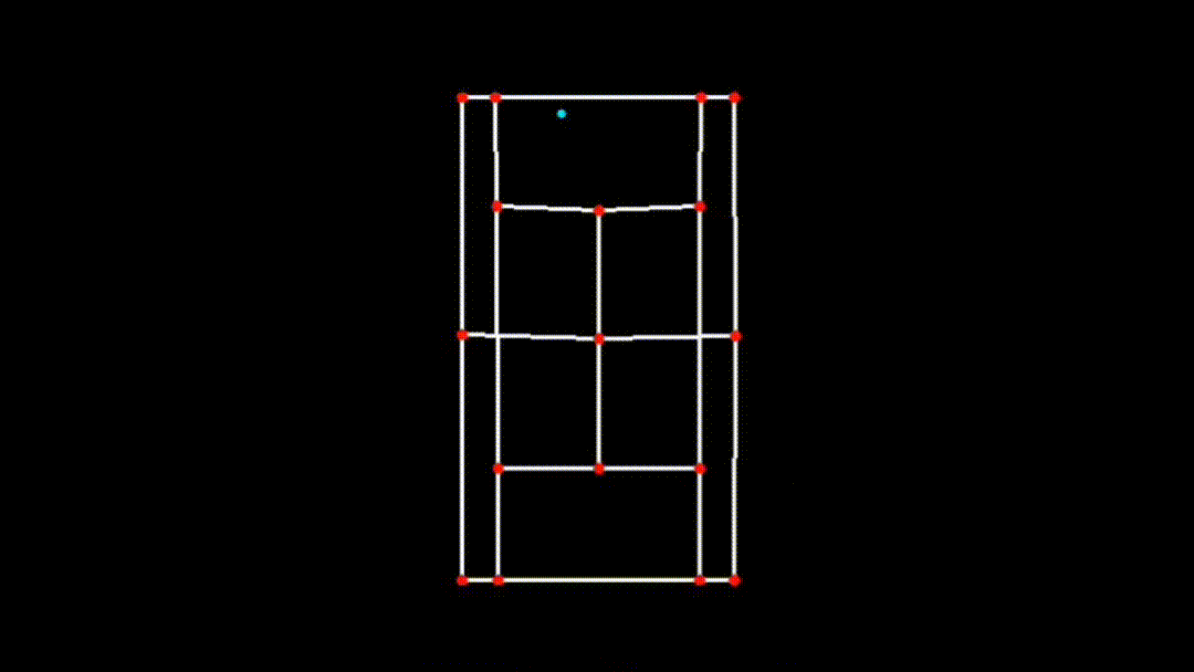
b. 📐 Transforming the Court into a 2D Plane Using Homography
After visualizing the court on the main frame, the next step is to transform these detected key points into a 2D, top-down view of the court. This transformation is essential for accurate analysis of the ball's position in relation to the court lines.
i. Homography Transformation
Homography Transformation is a mathematical technique used to map points from one plane to another, such as transforming the court from the camera’s perspective view to a top-down 2D view. In this project, homography transformation is crucial because it allows us to create an accurate 2D representation of the court, which is necessary for determining ball positions and making in/out calls.
ii. Extracting and Preparing Data for Transformation
The process starts with extracting the key points as discussed earlier. These key points are then used to define the court’s boundaries in both the original perspective and the target 2D plane.
src_points = np.array(
    [
        keypoint_dict["BTL"],  # Bottom-Top-Left
        keypoint_dict["BTR"],  # Bottom-Top-Right
        keypoint_dict["BBL"],  # Bottom-Bottom-Left
        keypoint_dict["BBR"],  # Bottom-Bottom-Right
    ],
    dtype=np.float32,
)

dst_points = np.array(
    [
        [black_frame_width // 6, black_frame_height // 7],  # BTL in 2D
        [black_frame_width * 5 // 6, black_frame_height // 7],  # BTR in 2D
        [black_frame_width // 6, black_frame_height * 6 // 7],  # BBL in 2D
        [black_frame_width * 5 // 6, black_frame_height * 6 // 7],  # BBR in 2D
    ],
    dtype=np.float32,
)src_points: These are the coordinates of the key points in the original frame, representing the four corners of the court.dst_points: These are the coordinates where these points should be mapped in the 2D plane. They represent where the corners of the court should be in the top-down view.
iii. Computing the Homography Matrix
The homography matrix is then computed using the source and destination points:
matrix = cv2.getPerspectiveTransform(src_points, dst_points)
transformed_keypoints = cv2.perspectiveTransform(keypoints[None, :, :2], matrix)[0]cv2.getPerspectiveTransform: This function calculates the homography matrix that maps src_points to dst_points.cv2.perspectiveTransform: This function applies the homography matrix to the key points, transforming them from the original perspective view to the 2D plane.
The result is a set of transformed key points that represent the court in a top-down 2D view.
iv. Visualizing the 2D Court
Finally, the transformed key points are used to visualize the court in 2D:
court_skeleton = visualize_2d(
    transformed_keypoints, lines, black_frame_width, black_frame_height
)
This function draws the court lines and boundaries based on the transformed key points, providing a clear and accurate 2D representation of the court.
| Transposed 2D Plane |
|---|
 |
This 2D transformation is a crucial step in ensuring the accuracy and effectiveness of the CourtCheck system, enabling precise in/out calls and detailed match analysis.
3. 🎾 Ball Tracking
Ball tracking is a critical component of CourtCheck, as it allows for precise analysis of tennis ball movements in relation to the court boundaries. The ball tracking model used in this project is TrackNet, an advanced deep learning model designed specifically for this purpose. The model's robust capabilities enable accurate tracking of the ball across frames, even in fast-paced tennis matches. The TrackNet model used here is adapted from yastrebksv's TrackNet implementation on GitHub.
a. 🛠️ How TrackNet is Integrated
The integration of TrackNet with the existing court detection pipeline ensures that both the court and ball movements are accurately represented in each frame of the video. Here’s a breakdown of how the ball tracking model is used, and how its output data is manipulated and visualized:
i. Loading and Using the TrackNet Model
TrackNet is loaded and applied to each frame to detect the ball's position. The model takes in a sequence of frames and outputs the predicted coordinates of the ball.
x_pred, y_pred = detect_ball(tracknet_model, device, frame, prev_frame, prev_prev_frame)
ball_track.append((x_pred, y_pred))detect_ballFunction: This function uses the TrackNet model to predict the ball's position(x_pred, y_pred)in the current frame based on the current and previous frames.- Frame Sequence: TrackNet utilizes a sequence of three consecutive frames (current, previous, and the one before that) to predict the ball's position, helping it account for the ball's movement across time.
The predicted ball position is then stored in ball_track, a list that accumulates the ball's trajectory over time.
ii. Visualizing Ball Movement on the Main Frame
Once the ball's position is detected, it is visualized directly on the main video frame. This visualization involves drawing circles on the frame to represent the ball's trajectory.
if x_pred and y_pred:
    for j in range(min(7, len(ball_track))):
        if ball_track[-j][0] is not None and ball_track[-j][1] is not None:
            if 0 <= int(ball_track[-j][0]) < processed_frame.shape[1] and 0 <= int(ball_track[-j][1]) < processed_frame.shape[0]:
cv2.circle(processed_frame, (int(ball_track[-j][0]), int(ball_track[-j][1])), max(2, 7 - j), (255, 255, 0), -1)- Ball Trajectory Visualization: Circles are drawn on the frame at the detected ball positions. The size of the circles decreases for previous positions, providing a visual trail of the ball's movement.
- Color and Positioning: The color
(255, 255, 0)is used for the circles, and the positions are carefully checked to ensure they fall within the frame’s boundaries.
iii. Transforming Ball Position to the 2D Plane
After visualizing the ball's trajectory on the main frame, the next step is to map the ball's detected position onto the 2D plane of the court. This is done using a homography matrix, which was previously computed during court detection.
if x_pred and y_pred:
    ball_pos_2d = transform_ball_2d(x_pred, y_pred, matrix)
    if 0 <= int(ball_pos_2d[0]) < court_skeleton.shape[1] and 0 <= int(ball_pos_2d[1]) < court_skeleton.shape[0]:
cv2.circle(court_skeleton, (int(ball_pos_2d[0]), int(ball_pos_2d[1])), 3, (255, 255, 0), -1)-
transform_ball_2dFunction: This function applies the homography matrix to the ball's position, transforming it from the original perspective view to the 2D top-down view of the court using OpenCV'scv2.perspectiveTransform(ball_pos, matrix)function.-
Transformation Process: The function first converts the ball's position
(x_pred, y_pred)into a format suitable for transformation(ball_pos = np.array([[x, y]], dtype=np.float32).reshape(-1, 1, 2)). -
Application of Homography Matrix: The
cv2.perspectiveTransformfunction then applies the homography matrix to this position, resulting intransformed_ball_pos, which represents the ball's position in the 2D plane. -
Visualizing in 2D: The transformed ball position is then drawn on the 2D court skeleton using a circle, ensuring that the ball's movement is accurately represented relative to the court boundaries in the 2D plane.
-
iv. Combining and Finalizing the Visualization
Finally, the court skeleton (with the ball's 2D position) is overlaid onto the processed main frame, and the combined frame is stored for generating the final output video.
processed_frame[0 : court_skeleton.shape[0], 0 : court_skeleton.shape[1]] = court_skeleton
combined_frames.append(processed_frame)- Overlaying the 2D Court: The processed frame now contains both the main frame visualization (with the court and ball trajectory) and the 2D court skeleton (with the ball’s position in the 2D plane).
- Frame Storage: The combined frame is added to the
combined_frameslist, which holds all the processed frames for the final video output.
🏆 Outcome
By integrating TrackNet with court detection, CourtCheck provides a comprehensive analysis of tennis matches. The system not only visualizes the ball’s movement relative to the court boundaries in the original video frame but also offers a clear 2D simulation of the court. This dual representation is essential for accurate in/out calls and for providing insights into ball trajectories during the match.
The combination of these techniques ensures that every aspect of the ball's movement is accurately captured and visualized, making CourtCheck a powerful tool for tennis match analysis.
The TrackNet model used in this project is credited to yastrebksv. Their implementation provided the foundation for the ball tracking functionality integrated into this project.
🪴 Areas of Improvement
- Accuracy: Enhance the accuracy of ball and court detection to ensure reliable analysis.
- Real-Time Processing: Implement real-time video feed analysis for instant decision-making during matches.
- Automatic Court Detection: Automate the court detection process to handle different court types and angles without manual input.
- Player Tracking: Integrate player tracking to provide comprehensive match statistics and insights.
🚀 Further Uses
- Match Analytics: Utilize the system for detailed match analytics, including player performance and shot accuracy.
- Training and Coaching: Provide coaches and players with valuable data to improve training sessions and match strategies.
- Broadcast Enhancement: Enhance sports broadcasting with real-time analysis and insights for viewers.
💻 Technology
- OpenCV: For image and video processing.
- Detectron2: For keypoint detection and court boundary identification.
- TrackNet: For tennis ball detection and tracking.
- NumPy: For numerical computations and data manipulation.
- PyTorch: For building and training machine learning models.
- tqdm: For progress bar visualization in loops and processing tasks.
🛠️ Installation
To set up the project, clone the repository and install the dependencies using the requirements.txt file:
git clone https://github.com/AggieSportsAnalytics/CourtCheck.git
cd CourtCheck
pip install -r requirements.txt
After installing the requirements, navigate to the scripts/process_video.py directory. At the bottom of the script, update the video paths to your desired input and output locations:
video_path = "..."  # Input Video Path (mp4 format)
output_path = "..."  # Output Video Path (mp4 format)
⚠️ Note: This process is for post-processing, meaning it will infer on a video input to detect the court and the ball. This operation is intensive on computer hardware and may take quite a bit of time to complete. If you want to use Google Colab's online GPU/processor instead, then head to Google Colab Notebook. Make sure to run all cells in chronological order.